Lesson 6
Overview
About Lesson 6
It really can't be said enough: HR diagrams are incredibly useful tools when studying stars. When we first studied HR diagrams, we identified different classes of stars—including white dwarfs, red giants, and main sequence stars—based solely on their inferred properties (e.g., radii). In this lesson, we are going to connect these different classes of stars with a single evolutionary track to continue in our pursuit of the story of stellar evolution. We will describe the physical changes going on within these stars that cause the observable changes reflected in their location in the HR diagram.
What will we learn in Lesson 6?
By the end of Lesson 6, you should be able to:
- Qualitatively describe the process of evolution for both low mass and high mass stars;
- Compare and contrast the stellar remnants of high and low mass stars;
- Describe the difference between variable stars and non-variable stars.
What is due for Lesson 6?
Lesson 6 will take us one week to complete.
Please refer to the Calendar in Canvas for specific time frames and due dates.
There are a number of required activities in this lesson. The chart below provides an overview of those activities that must be submitted for Lesson 6. For assignment details, refer to the lesson page noted.
| Requirement | Submitting your work |
|---|---|
| Lesson 6 Quiz | Your score on this quiz will count towards your overall quiz average. |
| Discussion: Black Holes | Participate in the Canvas Discussion Forum: "Black Holes". |
Questions?
If you have any questions, please post them to the General Questions and Discussion forum (not email). I will check that discussion forum daily to respond. While you are there, feel free to post your own responses if you, too, are able to help out a classmate.
The Transition to the Red Giant Phase for Sun-like stars
Additional reading from www.astronomynotes.com
Reminder!
Whenever you are considering the physical state of a star, you should separately consider its core (where the temperature and pressure are very high) and its envelope (where the temperature and pressure are substantially lower). The core is where fusion occurs, but the envelope is what we observe, so we have to infer what is going on in the core by observations of the envelope.
The most important concept to recall when studying stars is the concept of hydrostatic equilibrium. When nuclear fusion is going on in a star's core, the pressure created by this process pushes outward and balances exactly the inward pull of gravity. The first stage of the evolution of a star is the Main Sequence stage, and this accounts for approximately 80% of the star's total lifetime. During this time, the star is fusing hydrogen in its core. The star's color (a measurement of its surface temperature) and luminosity only change slightly over the course of its Main Sequence lifetime as the rate of nuclear fusion changes as the star slowly converts hydrogen to helium. When the star initially begins fusing hydrogen it is said to be on the Zero Age Main Sequence (ZAMS). Over a star's Main Sequence lifetime, as it fuses hydrogen into helium, its outer envelope will respond to slow internal changes, so its position in the HR diagram is not completely fixed. For example, we expect our Sun to brighten and its color to vary slowly over its roughly 10 billion year lifetime on the Main Sequence. By the end of its Main Sequence lifetime, it will be approximately twice as luminous as it is now!
When any star has used up the majority of the hydrogen in its core, it is ready to leave the Main Sequence and begin its subsequent evolution. From here on out, we will be considering the post-Main Sequence evolution for different types of stars. During the Main Sequence phase, core hydrogen fusion creates the pressure (in the form of radiation pressure and thermal pressure) that maintains hydrostatic equilibrium in a star, so you should expect that when a star's core has become filled with helium and inert, the star will fall out of equilibrium. As the total pressure decreases, gravity will once again dominate, causing the star to begin to contract again. You should be able to predict that when a stellar core contracts, its temperature will increase. So the star will continue to generate energy in its core, even when core hydrogen fusion ends, through the gravitational contraction of the core. Although fusion has turned the hydrogen in the core into helium, most of the outer layers of the star are made of hydrogen, including the layer immediately surrounding the core. Thus, when the core reaches a critical density and temperature during its contraction, it can ignite hydrogen fusion in a thin shell outside of the helium core. The helium core will also continue to generate energy by gravitational contraction, too. If you think of the Main Sequence as the “hydrogen core fusion” stage of a star's life, the first stage after the Main Sequence is the hydrogen shell fusion stage. During this stage, the rate of nuclear fusion is much higher than during the Main Sequence stage, so clearly the star cannot stay in this stage as long. For a star like the Sun, it will only remain in this stage for a few hundred million or a billion years, less than 10% of the Sun's Main Sequence lifetime.
While these internal changes are occurring in the star, its outer layers are also undergoing changes. The energy being generated in the core will be more intense than during the core hydrogen fusion (Main Sequence) phase, so the outer layers of the star will experience a larger pressure. The increased pressure will cause the outer layers of the star to expand significantly. As a side effect of this expansion, the outer layers of the star will cool down because they are now farther away from the energy source (the hydrogen shell around the core). The observable changes in the outer layers of the star will occur in two phases. First, the star will appear to cool slowly and will undergo a modest increase in luminosity. During this phase, the path the star will follow in the HR diagram is almost horizontal to the right of its position on the Main Sequence. Stars in this phase are usually referred to as subgiants. Next, the star will grow to as much as, or even more than, 100 times its original size, which will cause a significant increase in luminosity with only a small decrease in temperature, so the star will move almost vertically in the HR diagram. Stars in this area of the HR diagram are usually referred to as red giants. The evolutionary track for the star as it undergoes the transition to a red giant is shown below:

If you look at the dashed lines in this HR diagram, they represent lines of constant radius. When a star has reached the tip of the red giant branch (the highest point in luminosity on the track above), it has a radius of approximately 100 solar radii. There are several well known red giant stars even larger than this, which have radii of several hundred solar radii. The immense growth expected in the Sun when it becomes a red giant will cause its radius to swell from roughly 1 AU to perhaps 2 AU or so. This means that Mercury and Venus will definitely be engulfed by the Sun, and the Earth and Mars are likely to be engulfed as well. The core of the Sun when its envelope is 1 AU will only be of order 10 Earth radii, or a factor of more than 2,000 times smaller than the radius of the envelope.
Compare the illustrations below: the first shows the Sun as a red giant and compares it to the Sun at its current size (Fig. 6.2), and the second shows the measured size of Betelgeuse (Fig. 6.3).


Test this with Starry Night!
Your naked eye is not usually capable of making out the color of stars. One exception to this, though, is for the very bright red giant stars. If you are not already familiar with the night sky, find the following stars in Starry Night, and then try to find them by eye in your night sky. Note their color compared to the other stars visible in the sky (note, not all of these are visible at all times of year):
- Betelgeuse
- Aldebaran
- Arcturus
- Antares
In Lesson 5, you learned that the Main Sequence is a sequence in mass. That is, the hottest, brightest stars (O, B type) on the Main Sequence are also the most massive stars. The coolest, faintest (K, M type) stars on the Main Sequence are the least massive. Therefore, just by locating a star's position on the Main Sequence in the HR diagram, we can infer a reasonable estimate for its mass. All stars go through a red giant phase and wind up in the same general location in the HR diagram. Thus, we cannot infer the mass of a red giant star simply based on its location in the HR diagram. The track presented above is appropriate for Sun-like stars, but for more massive stars, their evolution proceeds a bit differently. After the red giant phase, the evolution of stars depends much more strongly on their initial mass, so we will have to consider stars of different masses separately from here on out. We will finish our discussion of Sun-like stars before we move into a discussion of more massive stars, like Betelgeuse.
The Final Stages of the Evolution of a Sun-like Star
Additional reading from www.astronomynotes.com
- Stellar Evolution Stage 6: Core fusion
- Stellar Evolution Stage 7: Red giant or supergiant
- Stellar Remnants
After the red giant phase, low mass stars follow a different evolutionary path than more massive stars. For this reason, we are going to first consider what happens to low mass (less than 8 times the mass of the Sun) stars as they progress past the red giant phase. To really study and understand stellar evolution in detail, you would want to subdivide stars more finely. That is, you would want to separately consider the evolution of stars of 0.1, 0.5, 1.0, 1.5, 2.0, 3.0, 5.0, and 8.0 solar masses, for example, and you would find differences between each. We are going to continue using a solar mass star as our example for low mass stellar evolution, but you should realize that the details of the evolution of stars of 0.5 solar masses or 5.0 solar masses deviate from the general description presented below.
During the red giant phase of a star's lifetime, the core is not in equilibrium. All of the fusion is occurring in a shell outside of the helium core, so there is no energy generation or outward radiation pressure to support the helium core. For this reason, the core of the star continues to collapse during the red giant phase. Collapse means an increase in temperature and density in the core. In many low mass stars (from about 0.5 - 3.0 solar masses), the core can be compressed to the point that it becomes a degenerate gas. This has important consequences in stellar evolution, so I will briefly describe what this means.
The gas inside stars is a soup of atomic nuclei and free electrons. If you compress a gas of this type to a high enough density, you have to use two of the laws of quantum mechanics to describe its behavior. These say:
- Like electrons bound in an atom, the free electrons can only have certain energies that you can represent as energy levels similar to the energy level diagrams we used in our study of the Bohr model of the atom.
- No two identical electrons can be found in the same energy level (the Pauli Exclusion Principle). Electrons can have two different spins, which each have a slightly different energy, so you can have two and only two electrons per energy level, one with spin up, the other with spin down.
The net effect of these two quantum mechanical effects is that when the gas has been compressed to the point where many of the lower energy levels have been filled, it begins to resist compression. Even though the physical state is still that of a gas, it is harder to compress a degenerate gas than solid steel!
Want to learn more?
For more detail on degenerate gases, see Stellar Remnants at www.astronomynotes.com.
At some point after the core has become degenerate, the core temperature reaches approximately 100 million kelvin, creating the proper conditions for three helium nuclei to fuse together to form one carbon nucleus (these carbon nuclei can also fuse with an additional helium nucleus to form one oxygen nucleus). This is referred to as the triple-alpha process, and it is an alternative fusion process to the proton-proton chain you learned about previously. In stars with degenerate cores, when this triple-alpha process begins, the entire core ignites at once in what is known as the helium flash. The star is now in the core helium fusion phase of its lifecycle. Contrary to what your intuition might tell you, in this phase, the outer layers of the star actually get smaller and hotter (the helium flash occurs in the core of the star in a very short time period and is not able to be observed directly). As you can see in the HR diagram below (Fig. 6.4), the evolutionary track of a Sun-like star now moves the star back towards the Main Sequence. This region of the HR diagram is called the horizontal branch, because stars in this phase of their evolution populate a narrow, almost horizontal box that extends to hotter temperatures from the red giant region of the diagram.

The horizontal branch phase of a star's life is much shorter than the Main Sequence phase of its lifetime. The star will convert all of its core helium into carbon and oxygen, and then fusion will end once again. The core will again begin to collapse inward with no radiation pressure to support it. Because there is still so much helium and hydrogen outside of the core of the star, after core helium fusion ends, the increased temperature can once again ignite shell helium fusion just outside of the carbon/oxygen core, and shell hydrogen fusion can continue outside of the helium shell. During this second phase of shell fusion, the outer layers of the star will expand again, but this time by an even larger amount. In this phase, the star can be called an asymptotic giant branch star, or sometimes a red supergiant star. For example, the star Antares is an M type supergiant. It has a luminosity 13,000 times that of the Sun.
For low mass stars, this is the final stage of their lifetime in which they generate energy via fusion. Once the helium and hydrogen shell fusion uses up all of the available fuel, the star's life is effectively over. However, the star will still leave behind two visible remnants. In the following table (6.1) we summarize some of the properties of a typical Sun-like star during its energy-generating lifetime:
| Evolutionary Stage | Duration | Temperature | Spectral Type | Luminosity | Radius |
|---|---|---|---|---|---|
| Main Sequence | 1010 years | ~6000 K | G | 1 LSun | 1 RSun |
| Red Giant | 109 years | ~3000 K | K - M | ~2000 LSun | ~150 RSun |
| Horizontal branch | 108 years | ~4500 K | G - K | ~100 LSun | ~20 RSun |
| Asymptotic Giant branch | 107 years | ~3000 K | K - M | ~10,000 LSun | ~200 RSun |
There is one last property of stars to consider, because it plays a more significant role as stars age; this is the stellar wind.
In this movie, we see an artist's impression of the solar wind, which is the stream of high energy particles being emitted by the Sun's corona. During the Main Sequence lifetime of Sun-like stars, this wind is not very strong—that is, the total amount of mass being lost by the Sun is small. However, during the later phases of a star's evolution, the mass loss rate associated with the stellar wind can increase significantly. By the time of the helium flash, a Sun-like star of initial mass 1.0 MSun may have only 0.7 MSun remaining. By the time the star has completed its nuclear fusion, there will be a significant amount of expelled gas from its envelope in its immediate vicinity.
Planetary Nebulae and White Dwarfs
Additional reading from www.astronomynotes.com
When a star reaches the asymptotic giant branch (its second ascent up the red giant branch), the outer layers of the star are, in general, several AU away from the core. If you recall from our study of the force of gravity, the magnitude of the inward pull drops off like the distance squared. Thus, the outer layers are no longer bound very strongly by gravity to the core. Given our observations of planetary nebulae (described in more detail below), we can infer that at some point near the end of the lifetime of a low mass star, it sheds its outer layers entirely. What astronomers are still trying to determine, however, is exactly the mechanism or mechanisms that are responsible for causing the envelope to be expelled. There are multiple scientific models for the expulsion, including the one described at astronomynotes.com: we know that in the late stages of stellar evolution that dust grains (e.g., the "soot and sand" we talked about in dark nebulae) form in the atmospheres of very cool giant stars. The pressure exerted on these dust grains in the atmosphere by the photons emitted by the star may be enough to push the loosely bound envelope away from the star. So, at the end of the lifetime of a Sun-like star, there will be two remnants: its envelope and its core.
The remnant of the core: The White Dwarf
The core of the star is no longer undergoing nuclear fusion of any variety, so it is once again collapsing. When the core reaches a size approximately equal to that of the Earth (about 100 times smaller than its original size when it was fusing hydrogen), the collapse will stop. The core will eventually achieve a stable equilibrium when electron degeneracy pressure resists the collapse. During this new equilibrium state, though, no fusion is occurring, so the carbon/oxygen remnant of the stellar core will not generate any new energy. Instead, it will simply cool off slowly by radiating light, getting fainter and fainter until it no longer gives off enough light to be visible. This process can take billions or even trillions of years. While the object is still visible, it is called a white dwarf, and it occupies the lower left of the HR diagram because of its high temperature and faint luminosity. White dwarfs are much smaller than typical stars, and thus are one of the stellar remnants often referred to as compact objects. Subrahmanyan Chandrasekhar won the Nobel Prize in Physics in 1983 for his contributions to our understanding of stellar evolution, including the stability of white dwarf stars. Chandrasekhar showed that, theoretically, white dwarf stars are only able to remain in equilibrium resisting gravitational collapse if their mass is below 1.4 MSun. Above that mass, electron degeneracy pressure is no longer able to resist gravity. This upper limit of 1.4 MSun for the mass of a white dwarf is known as the Chandrasekhar Limit.
Want to learn more?
Check out the Chandra Observatory's page about their namesake, Subrahmanyan Chandrasekhar.
If you consider that the size of a white dwarf is about the size of the Earth and that it contains approximately the same amount of mass as the Sun, you should realize that the properties of the material that make up a white dwarf must be unusual. The density of a white dwarf is unlike anything on Earth. The density of a material is its mass divided by its volume, and this number gives you an estimate of how tightly packed the material is within the volume it occupies. The more tightly packed (the denser), the heavier the object will feel. For example, let's consider a sugar-cube-sized lump of lead and a sugar-cube-sized lump of cotton. The lead is much denser than the cotton, so if you hold both lumps in your hand, even though they are the same size, the lump of lead will feel heavier. White dwarf material is much denser than lead. A sugar-cube-sized lump of white dwarf will have a mass of about 2,000 kg, which weighs about 4,000 pounds in Earth's gravity. It is expected that the coolest white dwarfs actually crystallize, and since they are primarily made of carbon/oxygen, they are occasionally compared to enormous diamonds, as in this press release from the Center for Astrophysics.
Because they are no longer generating energy by fusion, white dwarfs can be thought of as the "embers" of dead Sun-like stars. In some textbooks, authors refer to the final state not as a white dwarf, but as a black dwarf, which is achieved when the white dwarf has cooled to the point where it is no longer radiating any light at all. However, the time it takes for a white dwarf to cool to become a black dwarf is longer than the age of the Universe, so there are no black dwarfs yet in existence. The coolest white dwarfs known have temperatures of less than 4,000 K, while the most massive, youngest white dwarfs have temperatures of approximately 100,000 K!
Below is an image from the Hubble Telescope that was part of a study to identify the faintest, coolest white dwarfs in a star cluster called M4. We can estimate the age of these white dwarfs based on simple models of how they cool. They are found to be around 12 - 13 billion years old, which is consistent with the age of the Universe as determined by other methods.

The remnant of the envelope: The Planetary Nebula
The white dwarf also plays a role in the fate of the ejected outer layers of the star. For a brief time, by the standards of stars (only about 50,000 years or so), the intense UV light emitted by the white dwarf is illuminating the material that used to be the outer layers of the star. This light ionizes the atoms in the gas. The electrons freed by the ionization process periodically recombine with the ions in the gas, emitting photons in the process and creating an emission line spectrum. So, the outer layers will glow brightly, creating an emission nebula that is referred to as a planetary nebula. This name is very misleading. The nebulae have nothing to do with planets. When the first few planetary nebulae were discovered by telescopes, they appeared disk-shaped and greenish (recall the green color comes from the bright lines of oxygen seen in these objects), similar to the planet Uranus. Astronomers called them planetary nebulae because of their observational similarity to Uranus, but we now know they are the remnants of dead stars and have nothing to do with planets.
In the image below of the Ring Nebula, note how the interior looks greenish. Also, note that the white dwarf remnant of the star's core is located in the center of the nebula.

The duration of the planetary nebula stage for stars can be estimated quite simply in the following way:
- From spectroscopy, the expansion velocities of planetary nebulae are estimated to be approximately 20 - 30 km/sec.
- We can use the standard right triangle technique to determine the physical size of a planetary nebula if we measure its angular size and its distance.
- If you calculate size / velocity, you can estimate how long a particular planetary nebula took to expand to its current size.
- For a typical planetary nebula, its radius is of order 1 light year, or 9.5 x 10¹² km. So 9.5 x 10¹² km / 25 km/sec = 3.8 x 10¹¹ seconds, which is approximately 12,000 years. The largest planetaries have ages determined in this way to be less than 50,000 years.
My opinion, which is shared by other astronomers, is that planetary nebulae are some of the most beautiful objects photographed by telescopes. The Hubble Space Telescope has taken many images of different planetaries, and I encourage you to look at some of the samples I link to below. Planetary nebulae images appear in many places, including occasionally in pop culture. The group “Pearl Jam” even used a Hubble Space Telescope image of a planetary nebula as the cover of their CD Binaural.
- Hubble: Cat's Eye Nebula
- Hubble: Red Rectangle Nebula
- Hubble: Helix Nebula
- Hubble: Hourglass Nebula (and Binaural CD cover image)
- Hubble: Eskimo Nebula
- Hubble: Spirograph Nebula
Like many of the topics that we have covered in this lesson, astronomers have been able to determine some of the details related to the formation of planetary nebulae, but this is another area of active research. One model that is successfully able to describe some of the structures and properties observed in planetary nebulae is sometimes called the colliding wind model. The idea is that the star is surrounded by slow-moving gas produced when it had a strong stellar wind. When the envelope has mostly been removed from the star—exposing the core—a higher velocity outflow is created. This high-velocity gas plows into the low-velocity gas in the stellar neighborhood. This collision compresses the gas at the interface between the two winds, and it is that gas that glows and produces the rings of emission we see in many planetary nebulae. In planetaries that show elongated or hourglass structures, it is possible that a dense structure around the star's equator, caused by perhaps a stellar companion, may collimate the fast wind into oppositely directed jets of gas rather than into a spherically symmetric wind.
Watch this!
- Hubblesite provides a brief video story called a "Hubble Minute - Helix Nebula: A New Twist" on the formation of structures in complex planetary nebulae. They also provide links for the individual pieces of the production, including the short animation of the formation of a planetary nebula.
- Hubblesite also has a second visualization called "The Formation of Planetary Nebulae" that shows a possible scenario for creating a "bipolar" planetary nebula in a binary star system.
Briefly, let's mention the fate of the lowest mass stars here -- they will not become red giants nor emit planetary nebulae. Instead, we predict they will transition from red dwarf Main Sequence stars directly to white dwarfs. However, this is purely a theoretical prediction, because the expected Main Sequence lifetime of a star of < 0.4 MSun is approximately 10 trillion years. So, no star < 0.4 MSun that has formed in the Universe has yet been around long enough to die!
The Evolution of Massive Stars and Type II Supernovae
The lifecycle of high mass stars diverges from that of low mass stars after the stage of carbon fusion. In low mass stars, once helium fusion has occurred, the core will never get hot or dense enough to fuse any additional elements, so the star begins to die. However, in high mass stars, the temperature and pressure in the core can reach high enough values that carbon fusion can begin, and then oxygen fusion can begin, and then even heavier elements—like neon, magnesium, and silicon—can undergo fusion, continuing to power the star.
The evolutionary track of a high mass star on the HR diagram is also different from that of low mass stars. An O star on the Main Sequence will cool and expand after it runs out of hydrogen in its core, but it will move almost horizontally towards the red supergiant region of the HR diagram as it goes from helium fusion to carbon fusion to oxygen fusion. It will not experience a helium flash. Although high mass stars can continue to fuse heavier and heavier elements, each fuel runs out more quickly than the previous one. So, it may fuse hydrogen on the Main Sequence for 10 million years, but it will only fuse helium for 1 million years, and it can only maintain carbon fusion for approximately 1,000 years. At some point, the fusion reactions will create iron in the core of the star, and when this occurs, the star has only minutes to live.

Just as in low mass stars where you find a carbon/oxygen core surround by a helium-fusing shell surrounded by a hydrogen-fusing shell, we expect the core of massive stars to build up in the same way, but to include many more layers, as seen in the cartoon below.

The reason that fusion of light elements produces energy to support a star is because of the “mass defect” we discussed when we studied the proton-proton chain. The product of hydrogen fusion (one helium nucleus) has less mass than the four hydrogen nuclei that created it. The extra mass has been converted into energy. Each fusion reaction of light elements in the core of a high mass star always has a mass defect. That is, the product of the reaction has less mass than the reactants. However, when you fuse iron, the product of iron fusion has more mass than the reactants. Therefore, iron fusion does not create energy; instead, iron fusion requires the input of energy.
When iron builds up in the core of a high mass star, there are catastrophic consequences. The process of fusing iron requires the star's core to use energy, which causes the core to cool. This causes the pressure to go down, which speeds up the gravitational collapse of the core. This causes a chain reaction: core collapses, iron fusion rate increases, pressure decreases, core collapses faster, iron fusion rate increases, pressure decreases, core collapses faster, iron fusion rate increases, etc., which causes the star's core to collapse in on itself instantaneously. After the core collapses, it rebounds. A large quantity of neutrinos get created in reactions in the core, and the rebounding core and the newly created neutrinos go flying outward, expelling the outer layers of the star in a gigantic explosion called a supernova (to be precise, a type II or core collapse supernova).
For a brief period of time, the amount of light generated by one star undergoing a supernova explosion is greater than the luminosity of 1 billion stars like the Sun. These explosions are so bright that they are visible at immense distances. If a nearby star were to undergo a supernova explosion, it would be so bright it would be visible during the daytime. In modern history, no supernova has gone off close enough to us to be visible during the daytime. However, both Tycho Brahe and Johannes Kepler observed naked-eye supernovae during their lifetimes. In 1987, a supernova went off about 50,000 parsecs away from us. Below is a ground-based telescope image of the supernova about 2 weeks after the explosion. Note how bright the exploding star (lower right corner) is compared to all of the rest of the objects in the image.

In the Hubble Space Telescope image below, we see the remnant of supernova 1987a, which appears as rings of glowing light.

This supernova remnant has been studied in incredible detail, and astronomers have watched the remnant change since it was first discovered in 1987. Hubblesite provides a mosaic of images of its changing appearance.
Our understanding of the fusion reactions in the cores of stars and of supernova explosions has taught us that, as Carl Sagan is quoted as saying, "We are all star-stuff, contemplating the stars.” What he means is that if you consider the chemical elements that make up the human body—including carbon, oxygen, nitrogen, and all of the elements heavier than helium—these basic building blocks of life were all created by stars!
The elements that are lighter than iron are created by fusion reactions inside of massive stars. After the core collapse, when the shockwave is moving outwards through the outer layers of the exploding star, very high temperatures are reached. These temperatures are high enough that elements heavier than iron are produced during the supernova. We have observed the signatures of these heavier, radioactive elements in the spectra of supernovae.
Not only do supernovae serve as the mechanism for the creation of these heavy elements, they also serve as the mechanism for their dispersal. Our Sun is a low mass star, so it will only ever create carbon and oxygen within its core. It will never achieve the conditions necessary to create iron. However, when we take a spectrum of the Sun, we see spectral lines from nitrogen, sodium, magnesium, iron, silicon, and even rare elements such as europium and vanadium. These elements observed in our Sun (and in many other stars) were created in ancient supernovae explosions. The elements got dispersed by the supernova explosion and became mixed in with the gas in molecular clouds. Thus, when the next generation of stars formed, the gas in the molecular cloud already contained some heavy elements. Since the Earth (and all of us!) are made of heavy elements, life as we know it would not be possible without the occurrence of supernovae prior to the formation of our Sun.
Watch this!
To coincide with a press release related to observations of a supernova, the Chandra X-ray Observatory team put out an animation of a core-collapse supernova (it's #9 on this page), including the dispersal of gas rich in heavy elements into the ISM after the explosion ends.
Accretion in Binary Systems and Stellar Outbursts
Additional reading from www.astronomynotes.com
In the previous lesson, you learned about the existence of binary stars, and you were asked to speculate on the evolution of binary stars. We are going to return to this topic and study the consequences of mass transfer in binary systems.
First, we will cover the definition of the Roche Lobe. In a binary star system, each star is exerting a gravitational force on any object with mass in its vicinity. You can define a region inside of which the gravitational force from star 1 is stronger than star 2 and vice versa. The volume of space inside of which matter feels a stronger pull from star 1 than star 2 defines the Roche Lobe for star 1, and the volume of space inside of which matter feels a stronger pull from star 2 than star 1 defines the Roche Lobe for star 2. Any matter inside the Roche Lobe of an object will be gravitationally bound to that object. The two Roche Lobes for stars in a binary system are approximately teardrop shaped, and they meet at a point known as L1, or the first Lagrangian point. At L1, the gravitational force from both stars is exactly equal, so matter can actually go from being bound to one star to the other by passing through the L1 point.
Want to Learn More?
- NASA puts satellites at the Lagrange points in the Earth / Sun orbital system and has links to more information about these orbital locations. For example, see the WMAP Mission website and the JWST Mission website.
- Neil DeGrasse Tyson from the Hayden Planetarium has an essay on the Lagrangian points in the Earth / Sun system.
In the image below, a calculation of the 3D shape of the Roche Lobes for a binary star system and the 2D projection of the 3D volume is presented. The L1 point is labeled.

If you have two stars that are both smaller than their Roche Lobes, then that type of binary is referred to as a detached binary, and the stars will not have a direct influence on each other's evolution. However, if one of the stars grows large enough that it fills its Roche Lobe, then the shape of that star will become distorted, and mass can be transferred from the distorted star through the L1 point to the companion star in the binary. This system is referred to as a semi-detached binary. Mass transfer in these types of binary star systems is an active research area at Penn State.
Watch this!
The Chandra X-Ray Observatory has a nice animation of a binary star system evolving from a detached to semi-detached state. (Quicktime movie, which may not play in all browsers)
An animation of the stages in the evolution of the Algol system is available from Professor Michael Gallis of Penn State Schuylkill. It shows:
- an initially detached binary;
- the 2D projection of the Roche Lobes around the two stars;
- the 3D volume enclosed by the Roche Lobes for the two stars;
- the more massive star evolving, filling its Roche Lobe, and then transferring mass to its companion;
- the companion star gaining mass from the initially more massive star from the transfer;
- the new Roche Lobe geometry after the transfer, which shows that the star that gained mass now has a larger Roche Lobe than its companion.
There is one additional possibility we can address: If both stars in a binary fill their Roche Lobes, then mass from both stars will not be gravitationally bound to one star or the other, but instead the two stars will be surrounded by a "common envelope" of gas. This is referred to as a common envelope or contact binary.

Because binary star systems can transfer mass between the stars in the pair, this can alter the evolution of the stars in the binary and give rise to new types of stars and new stellar phenomena beyond the ones we have studied so far. For example, when a white dwarf is bound to another star in a binary star system and mass streams from the companion star towards the white dwarf, it can accumulate in a disk (called an accretion disk) that surrounds the white dwarf.

If a nearby companion dumps matter onto a white dwarf in this way, suddenly the hot, carbon/oxygen white dwarf is covered in a layer of new fuel, since the accreted matter will contain mostly hydrogen. The white dwarf is so hot that it can cause the hydrogen shell to undergo nuclear fusion similar to the process by which the degenerate core in a red giant creates a helium flash. When the hydrogen shell ignites in this manner, the fusion occurs explosively, and the star brightens by up to 1 million times its normal luminosity in a very brief time. We call this explosion a nova. In some systems, this process can happen over and over again, creating “recurring novae” explosions. Below is an example of a recurring nova imaged by the Hubble Space Telescope.

The word nova comes from the Latin "nova stella" or new star, because if a white dwarf near enough to Earth undergoes a nova explosion, we can see a naked eye star where previously there was no star. For example, below is an image of a "new star" or nova that was visible to the naked eye in 1999.

Novae are not the only possible end states for white dwarfs accreting matter from their companions. If a massive white dwarf near the Chandrasekhar limit accumulates too much mass from its companion by way of accretion, it can explode as a “Type Ia” supernova. Because electron degeneracy pressure cannot support a star with a mass > 1.4 solar masses, a white dwarf that accumulates enough mass to raise it above this limit will also explode violently. The amount of light given off during a Type Ia supernova is very similar to that of a Type II core collapse supernova. However, the spectrum of this light is very different. The stars that create Type II supernovae still contain hydrogen, so we will see evidence for hydrogen in the spectrum of a Type II supernova. Since white dwarfs do not contain any hydrogen, the spectra of supernovae created when they explode will not exhibit any hydrogen lines. These types of supernovae have been in the news recently because of their utility in the study of cosmology, and we will revisit them in a later lesson. In early 2014, the nearest and brightest Type Ia supernova was discovered, and it was visible to even backyard telescopes and binoculars. More information about Supernova 2014J in the galaxy M82 is available at many sources, including Sky & Telescope magazine.
There are many other stellar phenomena (e.g., "X-ray bursters") and stellar types (e.g., "blue stragglers") that are either known to be or are speculated to be the result of mass transfer in binary star systems. We will look at several more examples beyond the novae and type Ia supernovae described on this page.
Neutron Stars and Pulsars
Additional reading from www.astronomynotes.com
For stars less than approximately 8 solar masses, the remnant of the core that is left behind after stellar evolution is complete is the white dwarf. Since the Chandrasekhar limit is 1.4 MSun, this means that the more massive stars in the range of, say, 4 - 8 MSun must lose most of their mass so that the white dwarf they leave behind is less than this limit. We have seen that we expect massive stars to explode in core collapse supernovae, and that white dwarfs in binary systems may also explode in supernova explosions. The next logical question to address is: What remnant is left behind (if any) after these supernova explosions? When the core of a star collapses at the beginning of a Type II supernova explosion, a neutron star is created. Neutron stars are the second type of compact object we will study in this course.
Inside the iron core of a high mass star, the electrons cannot exert enough electron degeneracy pressure to resist the collapse. Therefore, the electrons get compressed to the point that they merge with the atomic nuclei in the core of the star. This inverse beta-decay reaction between electrons and protons creates both neutrons and neutrinos (this is the source of the neutrinos that helped blow off the outer layers of the star in the supernova explosion). When the neutrons have been created, they begin to resist further compression, exerting “neutron degeneracy pressure,” which halts the collapse of the core.
The remnant of the core has become essentially one giant atomic nucleus made up of neutrons. The typical size of an object of this sort is only about 10 kilometers in radius, but it can contain more than 1.5 solar masses of material. If you calculate the density of a neutron star, it is astounding—one sugar-cube-sized lump has a mass of half a trillion kg, which weighs about 1 trillion pounds in Earth's gravity. You may be curious to know the equivalent of the Chandrasekhar limit for neutron stars. That is, what is the mass limit above which even neutron degeneracy pressure is not strong enough to resist gravitational collapse? There is no easy answer to this question, though. The best estimates are that neutron stars have an upper mass limit of about 3 MSun, but that value is uncertain.
The first white dwarf star to be observed was Sirius B when it was resolved and separated from its companion (Sirius A) in the 1860s by Alvan Clark. If you want to make the same comparison and ask when the first neutron star was observed optically, the answer is in the 1990s by the Space Telescope. The image is below. However, this was not the first neutron star known. That discovery was made in the 1960s using observations in a different part of the electromagnetic spectrum.

There is another peculiar property of neutron stars beside their density, and that is their rotation rate. Conservation of angular momentum tells us that the rate of angular velocity (how fast an object spins) multiplied by its radius is a constant. The best analogy for this physical effect that you are probably familiar with is that of a spinning ice skater. If the skater starts to spin with his or her arms outstretched, they will spin slowly. However, when they pull their arms in (and thus decrease their radius), they will spin faster. We have already discussed at least one context where stars work the same way, that is, during the collapse of a molecular cloud to create protostars. However, conservation of angular momentum is also relevant to neutron stars; before a star explodes when it has an enormous radius, it might rotate once per month. When it collapses down into a neutron star with a radius of 10 km, it will spin up so that it now rotates once per second.
Because of their small size, neutron stars do not radiate much thermal energy (remember L = 4π R2 σ T 4, regardless of how large T is, if R is only 10 km, L will be quite small, too). They are, therefore, not bright enough to be plotted on an HR diagram. However, neutron stars do produce light through a different mechanism, which gets emitted out of two spots: one near the North magnetic pole and one near the South magnetic pole of the star. As the star spins once per second, the two spots appear as twin, rotating beams of light, similar to the light from a lighthouse on Earth. If we happen to be in the path of the beams, we detect a “pulse” of light from the neutron star. The first neutron stars to be detected were observed by radio telescopes as regularly repeating pulses of radio light with periods of about 1 second. These objects are called pulsars, and they happen to be the neutron stars oriented such that the Earth lies in the path of their lighthouse beam.
Watch this!
- Chandra has produced an animation of a pulsar seen in X-rays.
- Because pulsars are observed by radio telescopes that detect the radio emission from these objects, people often think that astronomers "listen" to pulsars, rather than detect their light curves (remember from when we studied binary stars—a light curve is a plot of how the brightness of an object changes as a function of time). Although astronomers do not listen to pulsars, some astronomers have taken light curves from a sample of pulsars and converted them to sound so you can hear the difference in their rotation rates. See the Jodrell Bank Radio Observatory website on the astronomical detections of pulsars.
The story of the discovery of pulsars is a very interesting one. A female graduate student at Cambridge University named Jocelyn Bell was using a new radio telescope to study the way in which radio waves from distant objects “twinkled.” During her study, she identified several regularly repeating radio signals from celestial objects with periods of about 1 second. Originally, she considered that the signals might even be from extraterrestrial civilizations, so the objects were labeled “LGM” for little green men. However, it was soon realized that these might be neutron stars, and this hypothesis has since been supported with much additional evidence. Jocelyn Bell's thesis adviser, Anthony Hewish, was awarded the Nobel Prize for the discovery of pulsars. Many people believe that Jocelyn should also have been awarded the prize because of her central role in the discovery. If you would like to read more of this story, I encourage you to read Jocelyn's own version:
- Little Green Men, White Dwarfs or Pulsars?
- Here is one of many versions of her talking about the discovery, at a talk the author of this course attended in 1995.
Recall that the accretion of matter on a white dwarf in a binary system can lead to either a nova explosion or a supernova explosion. The next question is: What happens to neutron stars or pulsars in binary systems? There are two possibilities that are not necessarily exclusive. That is, one system can exhibit both behaviors.
- X-ray burster: When a neutron star accretes matter in a manner similar to a white dwarf, the accretion disk will get so hot that it steadily emits in the x-ray part of the spectrum. However, when enough matter accumulates on the surface and fusion ignites, you get a burst of x-rays, instead of a nova.
- Millisecond Pulsar: We expect that young pulsars should rotate about once a second or perhaps as many as ten times or so per second. However, we have discovered many pulsars with periods close to 1 millisecond, which is 0.001 seconds. This means they spin 200 - 700 times per second. Millisecond pulsars are found to be in binary systems, and it appears that the accretion of matter has pushed on the surface of the neutron star in the direction of its rotation, causing it to rotate faster. This can revive a dead pulsar by spinning it back up to the speed necessary to emit like a lighthouse again. Indeed, we find millisecond pulsars in globular clusters, indicating that they are probably more than 10 billion years old. You don't expect pulsars to last that long, so they must have been revived via accretion. NASA has produced an animation of just this effect.
A few final notes on neutron stars and pulsars:
- Not all neutron stars are visible on Earth as pulsars. The reasons are because
- the beam from the pulsar's poles may not sweep past Earth, or
- over time the pulsar will slow down and its magnetic field will weaken, so a neutron star will only act like a pulsar for about 10 million years.
- The supernova explosion that created the pulsar may have also given it a kick, so we have discovered pulsars moving through space with velocities of usually about 100 km/sec. However, recently one was found moving at more than 1,000 km/sec.
Want to learn more?
We will not discuss "gravitational waves" as a separate topic in this course. However, this is an area of frontier research where the first direct detection was announced in February, 2016. Prior to this, the first indirect evidence for gravitational radiation came from the discovery of the binary pulsar system, PSR 1913+16, and pulsars are likely to continue to play a role in this growing field. There are several places you can go for more information:
- The 1993 Nobel Prize in physics was awarded for the discovery of PSR 1913+16.
- The millisecond pulsar animation at Goddard is related to a story about gravitational waves.
- NASA was preparing a mission called LISA, the Laser Interferometer Space Antenna, to search for gravitational waves; however, plans for this mission are on hold.
- The Penn State Center for Gravitational Wave Physics has an excellent page of resources on the search for gravitational waves.
Black Holes
Additional reading from www.astronomynotes.com
Want to learn more?
Before we go any further, let me note that Penn State teaches an entire face-to-face course on black holes (ASTRO 130) at the University Park campus. While it is true that most of the topics we will cover in ASTRO 801 can be elaborated on much more than I have the time or space for in this course, I think this is especially true of the topic of black holes. So, while we are going to address them here, I think that, in particular with this topic, if you want more detail, you should consider following up with additional reading and study beyond what is in the course on this page.
On the ASTRO 130 website, Professor Brandt lists the required reading and suggested reading on this topic, and you can certainly do well starting there with his recommendations.
Observationally, we find most neutron stars are approximately 1.4 solar masses. Theoretically, neutron stars may exist up to about 3 solar masses. Why is there an upper limit?
Let us again consider a Type II, core-collapse supernova. The implosion of the star compresses the core until it becomes essentially one giant ball of neutrons with a density larger than any other material known. The neutron star is supported by neutron degeneracy pressure. The question is: How strong is neutron degeneracy pressure?
In the case of the most massive stars (maybe only stars more massive than say, 25 or even 50 solar masses), not even neutron degeneracy pressure can stop the collapse of the core. In this case, at least 3 solar masses worth of matter collapses into a single point with infinite density. This point is referred to as a singularity. At a distance of approximately 9 km from the singularity is a spherical region at which the escape velocity is exactly equal to the speed of light. What this means is that any object that reaches this distance from the singularity (usually referred to as the event horizon or Schwarzschild radius) can never escape, even if it were moving at the speed of light. Thus, even light cannot escape from this object, and it is for this reason we call it a black hole.
You can calculate the size of the event horizon for a black hole in the following way:
- The escape velocity for an object with mass M and radius R is:
- Set , the speed of light, and solve for R
- ; we call this the Schwarzschild radius or
For an object of mass :
The Schwarzschild radius scales linearly with mass, so a 30 solar mass black hole will have a radius of 90 km, and a 300 solar mass black hole will have a radius of 900 km.
Watch out for this misconception!
If you have seen just about any science fiction movie that mentions black holes, you probably picture a giant space vacuum cleaner sucking material into some vast whirlpool. There is actually a nice short bumper sticker saying you should keep in mind from here on out: Black Holes don't suck!
Black holes have mass and exert gravitational force on their surroundings, just like every other mass in the Universe. They do not have some special force that allows them to suck nearby stars into their event horizon. What is peculiar about black holes is that they are the only objects where their event horizon is outside their physical boundary, and when you get near this boundary, strange physical effects occur because of the strong gravitational field associated with these objects.
For more, you can get the "Bad Astronomer's" (Phil Plait's) list of 10 things you don't know about black holes.
Let's momentarily review some of the most basic aspects of Einstein's theory of relativity. In order to understand how light behaves in the universe, we need to consider both Einstein's theory of special relativity and general relativity. These can be summarized quickly in two statements, but both statements have far reaching consequences.
- Special relativity says that there is no experiment that can tell whether you are undergoing straight-line, constant velocity motion, or whether you are standing still and everyone else is moving.
- General relativity says that there is no experiment that can tell whether you are standing in a gravitational field or are undergoing a constant, straight line acceleration.
One of the consequences of general relativity is that it requires that space be curved in the vicinity of large masses. This means that if a photon of light passes close to the Sun, for example, it will not continue in a straight line, but it will be deflected by a small amount (see www.astronomynotes.com for a more detailed explanation). Another prediction of general relativity is that when light is emitted by a massive object, it should be redshifted. That is, a photon of light feels a gravitational attraction to the massive object, and it must expend some of its energy in order to escape from the object. Because the energy of a photon is proportional to its wavelength or frequency (remember, UV photons carry more energy than IR photons, for example), when the photon loses energy, it gets redder. This is the gravitational redshift, and it is different from the Doppler effect redshift we have studied earlier.
General relativity predicts that these strange effects (such as the deflection of starlight near a massive object, or the gravitational redshift) will be stronger when a photon of light encounters a stronger gravitational field. Thus, it is difficult to measure these effects for the Sun, for example, but in theory they should be easier to measure in the vicinity of a black hole.
Watch this!
One of the astronomers responsible for Astronomy Picture of the Day has produced a number of simulations of what you might see near a black hole because of the strong relativistic effects, called Virtual Trips to Black Holes and Neutron Stars:
- Watch "Approaching the Black Hole" and "Circling the Black Hole".
- Read the explanation for both movies.
There are a number of additional effects that an observer investigating a black hole from near its event horizon will experience. Two of these include:
- If you could get close enough to a black hole, you would experience strong tides. The difference in the gravitational pull from one side of a person to another near a black hole can be enormous. It is so strong that a person (and actually, even a star) is likely to be torn apart. This is referred to as "spaghettification." At YouTube, you can watch Astronomer Neil DeGrasse Tyson describe this process.
- If you did take a trip to the event horizon of a black hole, what would an outside observer see happening to you? Any light you emit will be progressively redshifted the closer you get to the black hole, so the observer would see your light source (say you are shining a red laser pointer at them) first appear as IR, then as microwave, and then as radio light, the closer you got to the event horizon. A related effect is time dilation—that is, to you as you approach the black hole, your watch would continue to tick off every second at the same rate. However, an outside observer would see your watch tick slower and slower and slower the closer you got to the event horizon. Actually, a stationary observer would never be able to see you cross the event horizon, because time slows down so much that the moment of you crossing the event horizon would seem to take an infinite amount of time to the observer.
Want to learn more?
There are many additional questions you and your students are likely to have about black holes. For two excellent resources presented in FAQ format, see:
From an astronomer's point of view, beyond these thought experiments about the nature of black holes, the questions we are often more interested in are: How might we detect these objects and how do they influence their environments? The first question you might ask is, have we ever directly detected a black hole? Below is an artist's illustration of one of the primary candidates.

We have found binary star systems where an O star (with a mass of approximately 25 solar masses) is orbiting a companion that has a mass of 6 - 10 solar masses. However, the companion does not appear to emit any of its own light. Theoretically, neutron stars should not be able to survive with masses greater than about 3 solar masses. So, if a binary star system contains an unseen companion with a mass of more than 3 solar masses, it may be a black hole. A handful of such objects exist. The most famous is an object called Cygnus X-1 (shown in the illustration above), which has even had a song written in its honor ("A Farewell to Kings—Cygnus X-1" by Rush). To investigate Cygnus X-1 and some of the effects described previously, there is an online, interactive tool for younger students who want to investigate black holes: "Black Holes: Gravity's Relentless Pull," created by the folks at hubblesite.org.
Try this!
- Go to "Black Holes: Gravity's Relentless Pull."
- After watching (or skipping) the introduction, click on "Journey to a Black Hole."
- Click on "The Voyage" tab at the top of the window.
- After reading the info there, click on "Begin Your Voyage."
- Choose Cygnus X-1 for a short simulated trip to this binary star system.
- Click on the "Up Close and Personal" tab at the top of the window.
- Choose "Show Questions and Experiments" at the bottom of the window.
- Go through as many of the questions and experiments as you would like, but, in particular, choose "Drop a Clock into a Black Hole" and "Fall into a Black Hole."
Additional Resources
The resources linked at the end of Lesson 5 are all still relevant to this lesson:
- There is a short movie on star formation and stellar evolution in the Hubblesite movie theater. It is part of the Hubble exhibit on Stars.
- Chandra has a great classroom ready set of materials on stellar evolution.
In addition, there are many resources related to the specific topics we studied here:
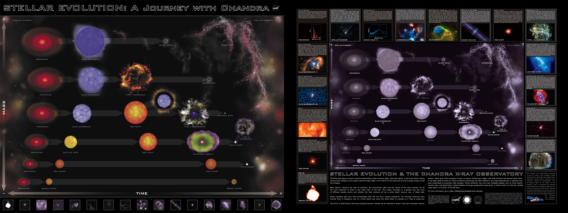
- Chandra has a full-sized poster that shows stellar evolution for all types of stars on one timeline. You can request a classroom copy.
- Goddard Space Flight Center's "Imagine the Universe" has a series of information and activity booklets related to topics from this and previous lessons:
- The first is called "The Lifecycle of Stars." It provides much of the background content seen in the last few lessons, but it also has associated classroom activities and demonstrations. I think you can still request a hardcopy of the booklet and associated poster from Goddard, too.
- The second is "The Anatomy of Black Holes," with background content and related activities. There is a K-8 and 9-12 version.
- Lastly, there is "What is Your Cosmic Connection to the Elements?".
- Although not everything is related to the topics here, you should investigate the entire "Teacher's Corner" at Imagine the Universe.
- NASA has been developing a supernova educator's resource guide, and the poster and guide are available for download.
- The NASA Fermi team has also put together a website full of black hole resources, including a black hole information sheet. Note that some of the links there overlap with links presented previously in this lesson (and in this list).
Summary & Final Tasks
This lesson contained a great deal of detail about the lives of stars, and yet there are still a number of topics that are left before we move on to galaxies. For now, though, you should hopefully have a detailed picture in your head about the process of star formation, evolution, and death for stars of all varieties.
Activity 1 - Lesson 6 Quiz
Directions
First, please take the Web-based Lesson 6 quiz.
- Go to Canvas.
- Go to the "Lesson 6 Quiz" and complete the quiz.
Good luck!
Activity 2 - Discussion
Directions
For this activity, I want you to reflect on what we've covered in this lesson and to speculate about black holes. Since this is a discussion activity, you will need to enter the discussion forum more than once in order to read and respond to others' postings.
Submitting your work
- Enter the "Black Holes" discussion forum in Canvas.
- Post your ideas about teaching the topic of black holes.
- Read postings by other ASTRO 801 students.
- Respond to at least one other posting by asking for clarification, asking a follow-up question, expanding on what has already been said, etc.
Grading criteria
You will be graded on the quality of your participation. See the grading rubric (identical to the one from Earth 530) for specifics on how this assignment will be graded.
Reminder - Complete all of the lesson tasks!
You have finished the reading for Lesson 6. Double-check the list of requirements on the Lesson 6 Overview page to make sure you have completed all of the activities listed there before beginning the next lesson.